Machine Learning – Page 5 – Margus Roo

Diskreetse juhusliku suuruse keskväärtus (EX) – R

Posted on April 26, 2013 - April 26, 2013 by margusja

Diskreetse juhusliku suuruse X keskväärtuseks (matemaatiliseks ootuseks) EX nimetatakse suuruse võimalike väärtuste ja nende tõenäosuste korrutiste
summat

Näide:

R-ga

* X väärtused (sündmus) y <- c(2, 3, 4, 5, 6, 7, 8, 9, 10, 11, 12);

* p väärtused (sündmuse tõenäosus) d <- c(1/36, 1/18, 1/12, 1/9, 5/36, 1/6, 5/36, 1/9, 1/12, 1/18, 1/36);

* Loome maatriksi z – z<-cbind(y,d)

> summary(z)

* Graafiline esitus

Võib tähele panna, et:

* Diskreetse juhusliku suuruse keskväärtus on ligikaudu võrdne katseseeria jooksul ilmnenud
juhusliku suuruse väärtuste aritmeetilise keskmisega ning sealjuures seda täpsemalt, mida
suurem on katsete arv.
* Kui viia läbi mitu katseseeriat, siis iga katseseeria jaoks leitud juhusliku suuruse väärtuste
aritmeetilised keskmised kuhjuvad konstandi ümber, milleks on selle juhusliku suuruse
keskväärtus.

Lineaarne regressioon

Posted on April 25, 2013 - April 25, 2013 by margusja

* Eelduseks on, et sõltuva ja sõltumatu (sõltumatute) muutuja (muutujate) vahel on lineaarne seos.

* Sõltuv muutuja – muutuja mida üritatakse ennustada ühe või enama sõltumatu muutuja kaudu

* Mida vähem sõltumatud muutujad omavahel korrelatsioonis on, seda parem. Võimalus eelnevalt tugevas korrelatsioonis olevad sõltumatud muutujad eemaldada.

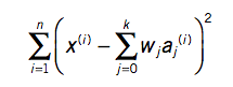
* Mudeli kvaliteeti saab mõõta “Root Mean Squared Error” valemiga, mille tulemus on 0 ja 1 vahel. Mida lähemal on see tulemus 0-le seda parem. Kirjeldab punktide kauguste summa ruutu lineaarsest joonest

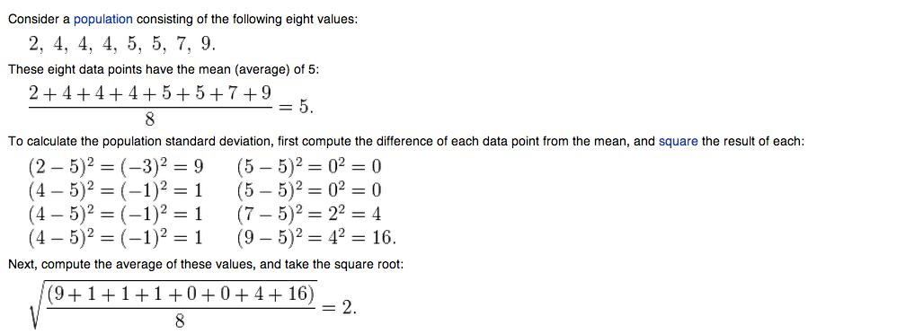
* Standard error – Standardviga (standard error, SE) ehk valimi keskväärtuse standardhälve on SD/pn. Formaalselt on tegu standardhälbega sellises uues üldkogumis, mis tekib, kui tegelikust üldkogumist võetakse uuritava valimiga võrdse suurusega valimeid ja arvutatakse uute valimite keskväärtused. Standardviga on siis selliste hüpoteetiliste valimite keskmiste standardhälve. Iseloomustab meie teadmiste täpsust uuritava üldkogumi keskmisest, mida täpsem on meie teadmine, seda väiksem on SE. SE sõltub seega a) üldkogumi dispersioonist; b) valimi suurusest. Mida suurem on valim, seda väiksem on SE. Valimi suurenedes läheneb SE nullile. See on siis oluline erinevus SD-st. Mida lähem 0-le, seda parem

* t-Stats – Mida kaugemal nullist, seda parem

* p-value – Mida lähemal nullile, seda parem.

* Student’s t-test is a method in statistics to determine the probability (p) that two populations are the same in respect to the variable that you are testing.

* Tolerance – the tolerance measures the influence of one independent variable on all other independent variables; the tolerance is calculated with an initial linear regression analysis. Tolerance is defined as T = 1 – R² for these first step regression analysis. With T < 0.1 there might be multicollinearity in the data and with T < 0.01 there certainly is

* p-value The p value is NOT a probability but a likelihood. It tells you the likelihood that the coefficient of a variable in regression is non zero.
The p-value is: The probability of observing the calculated value of the test statistic if the null hypothesis is true

p-values smaller than our chosen significance level (usually 0.05) indicate variables that should be in our final model.

P-values larger than our significance level may be left out of the model.

Nullhüpotees ( H0 või H0 ) – konservatiivne väide, mis eeldab tavaliselt, et muutusi ei ole, erinevus puudub jms.

Alati määratakse kindlaks ülempiir tõenäosusele teha esimest liiki viga. Taolist
ülempiiri nimetatakse olulisusenivooks ja tähistatakse (alfa, significance level).
Vähimat olulisusenivood, mille korral me saame alternatiivse hüpoteesi vastu võtta,
nimetatakse olulisustõenäosuseks ja tähistatakse p (significance probability, pvalue). Kui olulisustõenäosus on väiksem kui meie poolt valitud olulisuse nivoo,
võime H1 vastu võtta. Teaduskirjanduses on saanud tavaks valida =0.05 või 0.01.

Simple Standard deviation example

Posted on March 12, 2013 by margusja

Machine learning – erinevad kernelid

Posted on March 7, 2013 by margusja

Hea näide erinevatest kernelitüüpidest

Weka – mehed ja mood

Posted on March 7, 2013 by margusja

Wekas klasterdamise tulemusena selgus, et naiste vanuse kasvades nad tunnevad moetrendide vastu jätkuvalt huvi, mehed seevastu kaotavad moe vastu huvi vanuse kasvades

Machine learning basics

Posted on February 26, 2013 - August 12, 2015 by margusja

we should really talk of file mining rather than data- base mining – kuna me anname tihti mudeli tegemiseks ette denormaliseeritud flat data.

In classification learning, the learning scheme is presented with a set of classified examples from which it is expected to learn a way of classifying unseen examples.

Classification learning is sometimes called supervised

In association learning, any association among features is sought, not just ones that predict a particular class value .

Association rules differ from classification rules in two

ways: They can “predict” any attribute, not just the class, and they can predict more than one attribute’s value at a time.

Association Rules – Some rules imply others. To reduce the number of rules that are produced, in cases where several rules are related it makes sense to present only the strongest one to the user

When there is no specified class, clustering is used to group items that seem to fall naturally together.

In clustering, groups of examples that belong together are sought.

The success of clustering is often measured subjectively in terms of how useful the result appears to be to a human user

Numeric prediction is a variant of classification learning in which the outcome is a numeric value rather than a category.

In numeric prediction, the outcome to be predicted is not a discrete class but a numeric quantity. Input

The input to a machine learning scheme is a set of instances. These instances are the things that are to be classified or associated or clustered

Each instance that provides the input to machine learning is characterized by its values on a fixed, predefined set of features or attributes The value of an attribute for a particular instance is a measurement of the quantity to which the attribute refers

There is a broad distinction between quantities that are numeric and ones that are nominal. Numeric attributes, sometimes called continuous attributes, measure numbers—either real or integer valued.

Nominal attributes are sometimes called categorical, enumerated, or discrete – näiteks peretüüp, silmade värv, sugu.

a process of flattening that is techni- cally called denormalization Output

A linear regression

Linear models can also be applied to binary classification problems. In this case, the line produced by the model separates the two classes: It defines where the deci- sion changes from one class value to the other. Such a line is often referred to as the decision boundary.

Decision tree

In instance-based classification, each new instance is compared with existing ones using a distance metric, and the closest existing instance is used to assign the class to the new one. This is called the nearest-neighbor classification method. Sometimes more than one nearest neigh- bor is used, and the majority class of the closest k neighbors (or the distance- weighted average if the class is numeric) is assigned to the new instance. This is termed the k-nearest-neighbor method

Deriving suitable attribute weights from the training set is a key problem in instance-based learning

Methods

Naïve Bayes

Table shows a summary of the weather data obtained by counting how many times each attribute–value pair occurs with each value (yes and no) for play

Likelihood of yes = 2/9×3/9×3/9×3/9×9/14 = 0.0053

Likelihood of no = 3/5 × 1/5 × 4/5 × 3/5 × 5/14 = 0.0206

Tree

Outlook= sunny: info((2,3))= entropy(2/5,3/5) = -2/5 * log(2/5) – 3/5 * log(3/5) = 0.971 bits

Outlook = overcast: info((4,0)) = entropy(1,0) = -1 * log(1) – 0 * log(0) = 0 bits

Outlook = rain: info((3,2)) = entropy(3/5, 2/5) = -3/5 * log(3/5) – 2/5 * log(2/5) = 0.971 bits

Expected info for Outlook = Weighted sum of the above: info((3,2),(4,0),(3,2)) = 5/14 * 0.971 + 4/14 * 0 + 5/14 * 0.971 = 0.693

Pisike käsurea utiliit otsustuspuu genereerimiseks

Veel üks alternatiivne variant tree genereerimiseks

MINING ASSOCIATION RULES

Otsime nn ItemSet paare. Otsime paare, mis tekivad minimaalselt kahel tingimusel.

Näiteks üks kahele tingimusele vastav paar oleks Outlook=Sunny, Temperature=hot

Kolmene paar oleks Outlook= Sunny, Temperature=hot, Humidity=high

Neljase paari näide Outlook=Sunny, Temperature=hot, Humidity=high, Play=no

Kirjeldame, mitu paari me leiame. Näiteks neljast item-set paari (Outlook=Sunny, Temperature=hot, Humidity=high, Play=no) leiame kahel korral.

Saame alloleva tabeli

Genereerime reeglid

Võtame näiteks ühe kolmese paari – humidity = normal, windy = false, play = yes ja vaatame milliseid tingimusi sealt annab genereerida.

Lisaks paneme kirja mitu korda mingi tingimus esineb ja mitmel korral ta on tõene.

humidity = normal, windy = false, play = yes If humidity = normal and windy = false then play = yes 4/4 (iga paar annab play = yes / neli paari humidity = normal and windy = false e 4/4 – coverage) 4/4 = 1 ehk 100% accuracy If humidity = normal and play = yes then windy = false 4/6 ( 4 kord kuuest tingimusest humidity = normal and play = yes on tõene windy = false) 4/6 – coverage, (0.66) 70% accuracy If windy = false and play = yes then humidity = normal 4/6 If humidity = normal then windy = false and play = yes 4/7 If windy = false then humidity = normal and play = yes 4/8 If play = yes then humidity = normal and windy = false 4/9 If – then humidity = normal and windy = false and play = yes 4/14 – siin näiteks on tingimus humidity = normal and windy = false, mis ilmneb 14 korral ainult 4 korral tõene. Kui me nüüd seame tingimuseks et minimaalne coverage on 2 ja minimaalne accuracy = 100% siis saame 58 reeglit. Mõned neist allpoolt toodud tabelis

…

Weka solution to generate rules

Numeric Prediction: Linear Regression (supervised) Kui andmed on numbrilised/skalaarid, siis linear regression on üks meetoditest, mida kaaluda.

x=w0 +w1*a1 +w2*a2 +…+wk*ak x – class a0, a1,a2,…, ak – attribute values (a0 is always 1 – bias) w0, w1,…., wk – weights (are calculated from the training data)

The predicted value for the first instance’s class can be written as

antud valem ei anna mitte klassi väärtust vaid ennustatud klassi. Tuleb hakata võrdlema viga, mis on reaalse klassi ja ennustatud klassi vahel Erinevaid online linear regression tööriistasid on olemas (http://www.wessa.net/slr.wasp) Üks näide X, Y 1,1 1,2 2,1 2,3 2,4 4,3 4,4 wolfram alfa

Of course, linear models suffer from the disadvantage of, well, linearity

K-Nearest neighbors (supervised) training data and generated tree (k = 2 )

Clustering (unsupervised)

techniques apply when there is no class to be predicted but the instances are to be divided into natural groups

The classic clustering technique is called k-means

Support vector machines select a small number of critical boundary instances called support vectors from each class and build a linear discriminant function that separates them as widely as possible. This instance-based approach transcends the limitations of linear boundaries by making it practical to include extra nonlinear terms in the function, making it possible to form quadratic, cubic, and higher-order decision boundaries

e ja f on väga sarndased

The function (x • y)^n, which computes the dot product of two vectors x and y and raises the result to the power n, is called a polynomial kernel.

Other kernel functions can be used instead to implement different nonlinear mappings. Two that are often suggested are the radial basis function (RBF) kernel and the sigmoid kernel. Which one produces the best results depends on the applica- tion, although the differences are rarely large in practice. It is interesting to note that a support vector machine with the RBF kernel is simply a type of neural network called an RBF network (which we describe later), and one with the sigmoid kernel implements another type of neural network, a multilayer perceptron with one hidden layer.

Mathematically, any function K(x, y) is a kernel function if it can be written as K(x, y) = ?(x) • ?(y), where ? is a function that maps an instance into a (potentially high-dimensional) feature space. In other words, the kernel function represents a dot product in the feature space created by ?

Just one k-mean picture