Math – Margus Roo

Statistika ja katseseeria pikkus

Posted on July 31, 2017 - July 31, 2017 by margusja

Kasutades R keelt ja RStudio rakendust näitan, miks on katseseeria pikkus oluline.

Võtame näidisvektori:
> myFamilyAges
[1] 43 42 12 8 5

Antud vektori elementide keskmine (mean):
> mean(myFamilyAges)
[1] 22

Võtame nüüd sample() käsuga viis korda kõnealusest vektorist viis elemente ja arvutame nende keskmise:
> mean(sample(myFamilyAges, 5, replace = TRUE))
[1] 22.6
> mean(sample(myFamilyAges, 5, replace = TRUE))
[1] 35.8
> mean(sample(myFamilyAges, 5, replace = TRUE))
[1] 21.4
> mean(sample(myFamilyAges, 5, replace = TRUE))
[1] 13.2
> mean(sample(myFamilyAges, 5, replace = TRUE))
[1] 35.4

nagu näeme varieerub tulemus tugevalt:

> sd(c(22.6,35.8,21.4,13.2,35.4))
[1] 9.752538

Võtame nüüd ühe korra 4000 korda samast vektorist elemente ja arvutame nende keskmise:
> mean(sample(myFamilyAges, 4000, replace = TRUE))
[1] 21.8995

Kuvame ka tihedusgraafikud

Nagu näha – kohe väga lähedale originaalvektori keskmisele (22).

Seega – suurus on oluline 🙂

Üks miljonist

Posted on December 25, 2015 - December 25, 2015 by margusja

Kindlasti on tuttav väljend: “Üks võimalus miljonist.” Erinevad inimesed interpreteerivad eeltoodud lauset omamoodi.

Näiteks, kui ütelda, et lotovõidu tõenäosus on 1:1000 000, siis kas see tähendab, et kui miljon inimest mängib lotot, siis keegi kindlasti võidab? Ei? Tõsi – nii see päris ei ole, kuigi tihti seda nii lahti mõtestatakse. Aga kuidas suhet 1:1000 000 siis mõista?

Seletamiseks võtame natukene lihtsama skaala – täringu. Küsime: “Kui tõenäoline on, et kuue viske jooksul ei saa me kordagi kuut silma?” Arvutatakse seda järgnevalt: (1-(1/6))^6 e 1/6 on tõenäosus, et visatakse kuus iga eraldi katse käigus. 1- on vastassündmuse jaoks. Astendaja kuus on katsete arv. Selgub, et antud arvutuse tulemus on ligikaudu 0.33 e 1/3 on tõenäosus, et kuue viske jooksu ei tule kordagi kuus. Võis siis 2/3 on tõenäosus, et tuleb kuus.

Ülaltoodust saab üsna lihtsalt tuletada üldvalemi – P(newer) = (1-(1/n))^n

Kui nüüd antud funktsiooni kuju vaadata (Joonis 1.), siis selgub, et tõenäosus katsete arvu suurenemisel praktiliselt ei suurene e võib ka väita, et miljoni viskamise korral ei saa väga kindlalt väita, et kuus ikka tuleb.

Joonis 1.

Mis aga kõige lahedam. Aastal 1690 J. Bernoulli tegeles sama probleemiga ja avastas, et katsete väga suurel hulgal allub graafik palju lihtsamale valemile – 1/e

Allikas: https://www.countbayesie.com/blog/2015/2/18/one-in-a-million-and-e

Bitwise operations

Posted on September 9, 2015 by margusja

Bitwise operations are usually easier to CPU.

NOT

011 (3)

NOT 3 = 4 (100)

AND

011 (3) AND 100 (4) = 0 (000)

011 (3) OR 100 (4) = 7 (111)

Real life versus designed process

Posted on August 18, 2015 by margusja

Neural network

Posted on August 3, 2015 - August 5, 2015 by margusja

a = x1*w1 + x2*w2 + x3*w3 … xn*wn

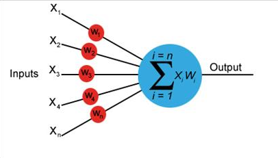
Feedforward newwork

In case we have matrix 8X8 we need 64 input

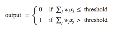
Threshold

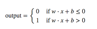
Bias

Learning

Learning rate = 0.1
Expected output = 1
Actual output = 0
Error = 1

Weight Update:
w_i = r E x + w_i
w₁ = 0.1 x 1 x 1 + w₁
w₂ = 0.1 x 1 x 1 + w₂

New Weights:
w₁ = 0.4
w₂ = 0.4

Learning rate = 0.1
Expected output = 1
Actual output = 0
Error = 1

Weight Update:
w_i = r E x + w_i
w₁ = 0.1 x 1 x 1 + w₁
w₂ = 0.1 x 1 x 1 + w₂

New Weights:
w₁ = 0.5
w₂ = 0.5

Learning rate = 0.1
Expected output = 1
Actual output = 1
Error = 0

No error,
training complete.

Lets implement it in Java
public class SimpleNN {

private double learning_rate;
private double expected_output;
private double actual_output;
private double error;

public static void main(String[] args) {

// initial
SimpleNN snn = new SimpleNN();
snn.learning_rate = 0.1;
snn.expected_output = 1;
snn.actual_output = 0;
snn.error = 1;

// inputs
int i1 = 1;
int i2 = 1;

// initial weigths
double w1 = 0.3;
double w2 = 0.3;

// loop untill we will get 0 error
while (true) {
System.out.println(“Error: “+ snn.error);
System.out.println(“w1: “+ w1);
System.out.println(“w2: “+ w2);
System.out.println(“actual output: “+ snn.actual_output);
w1 = snn.learning_rate * (snn.expected_output – snn.actual_output) * i1 + w1;
w2 = snn.learning_rate * (snn.expected_output – snn.actual_output) * i2 + w2;
snn.actual_output = w1 + w2;
if (snn.actual_output >= 0.99)
break;
}
System.out.println(“Final weights w1: “+ w1 + ” and w2: “+ w2);

}

Run it:
Error: 1.0
w1: 0.3
w2: 0.3
actual output: 0.0
Error: 1.0
w1: 0.4
w2: 0.4
actual output: 0.8
Error: 1.0
w1: 0.42000000000000004
w2: 0.42000000000000004
actual output: 0.8400000000000001
Error: 1.0
w1: 0.43600000000000005
w2: 0.43600000000000005
actual output: 0.8720000000000001
Error: 1.0
w1: 0.44880000000000003
w2: 0.44880000000000003
actual output: 0.8976000000000001
Error: 1.0
w1: 0.45904
w2: 0.45904
actual output: 0.91808
Error: 1.0
w1: 0.467232
w2: 0.467232
actual output: 0.934464
Error: 1.0
w1: 0.4737856
w2: 0.4737856
actual output: 0.9475712
Error: 1.0
w1: 0.47902848
w2: 0.47902848
actual output: 0.95805696
Error: 1.0
w1: 0.48322278399999996
w2: 0.48322278399999996
actual output: 0.9664455679999999
Error: 1.0
w1: 0.4865782272
w2: 0.4865782272
actual output: 0.9731564544
Error: 1.0
w1: 0.48926258176
w2: 0.48926258176
actual output: 0.97852516352
Error: 1.0
w1: 0.491410065408
w2: 0.491410065408
actual output: 0.982820130816
Error: 1.0
w1: 0.4931280523264
w2: 0.4931280523264
actual output: 0.9862561046528
Error: 1.0
w1: 0.49450244186112
w2: 0.49450244186112
actual output: 0.98900488372224
Final weights w1: 0.495601953488896 and w2: 0.495601953488896

So…Christopher CAN LEARN!!!

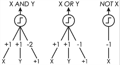
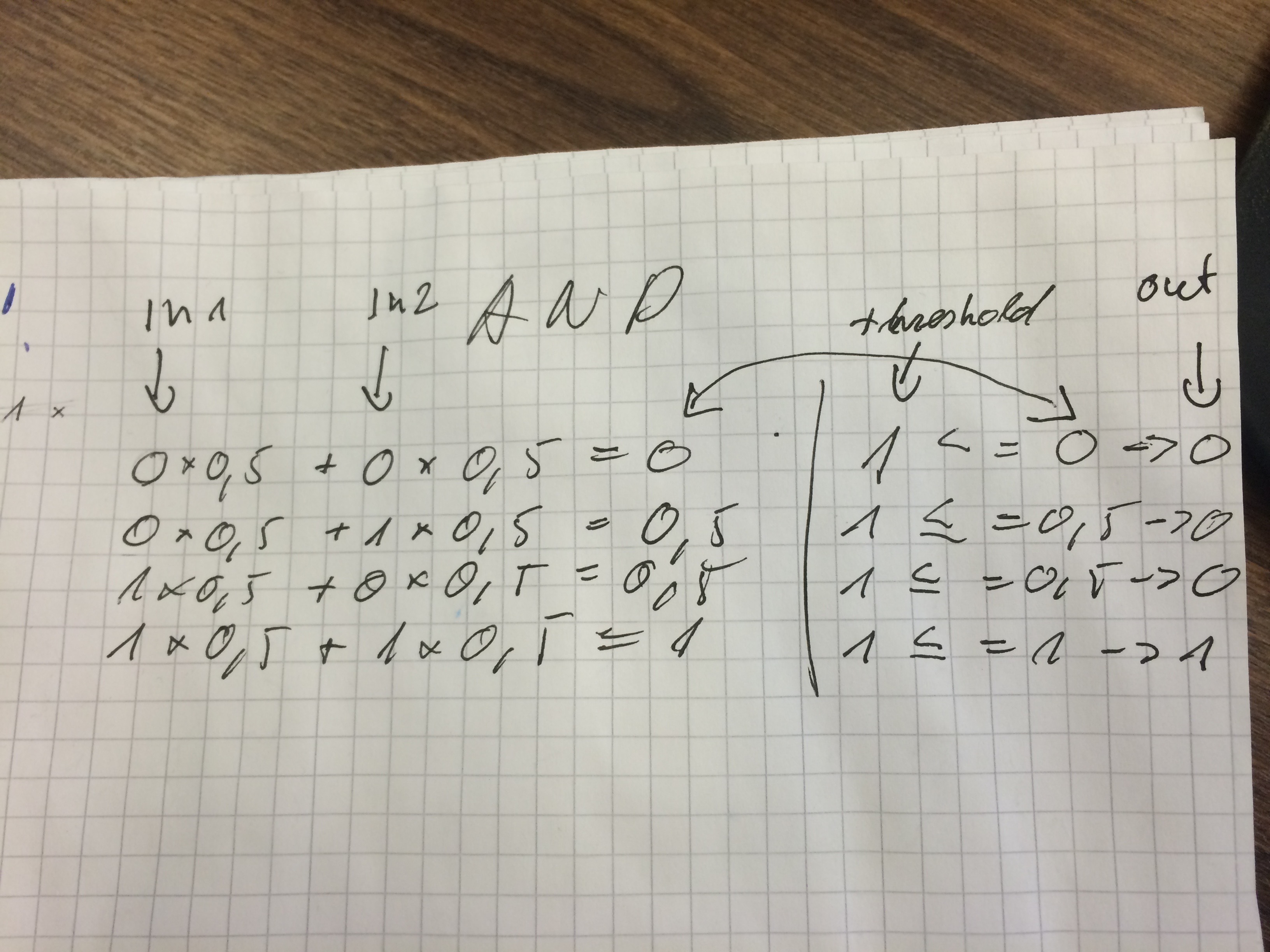
Neural network with AND logic.

0 & 0 = 0

0 & 1 = 0

1 & 0 = 0

1 & 1 = 1

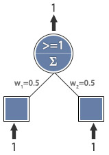
Using neural network you can use only one perceptron

In paper calculated weights and AND logic

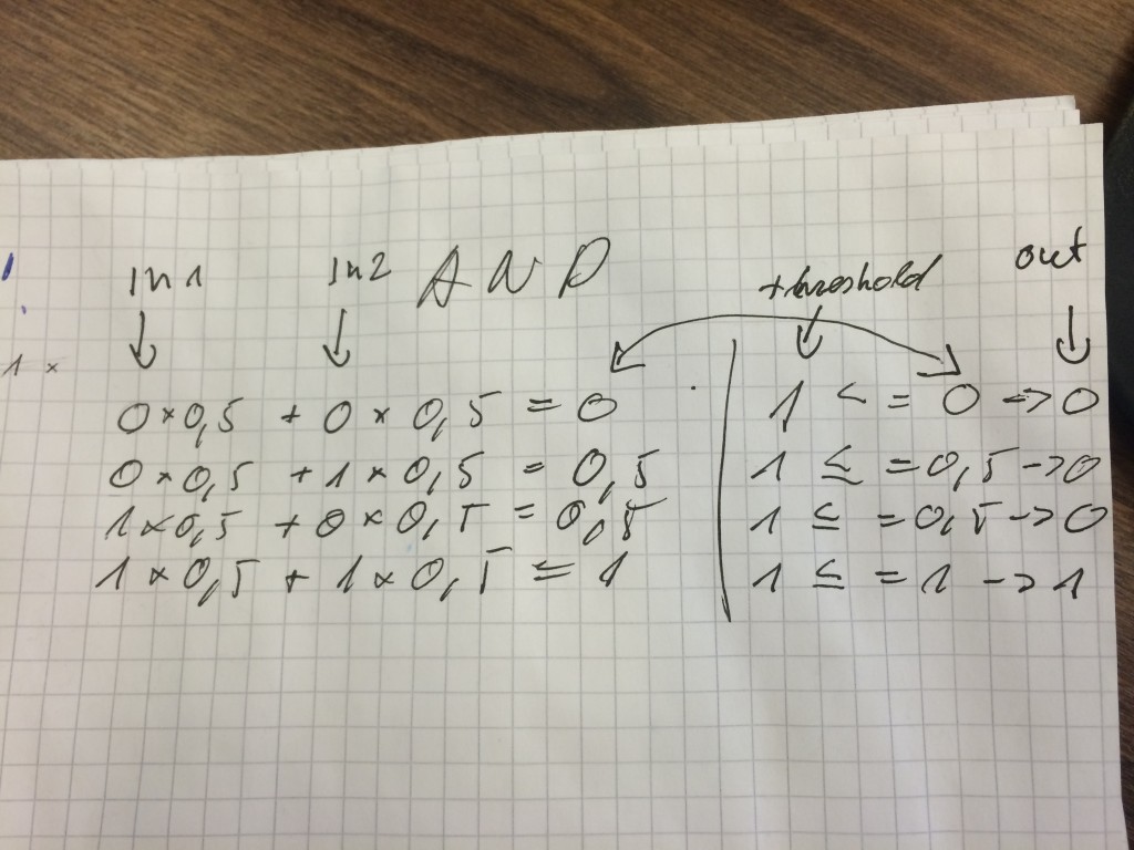
So we need to find weights fulfil conditions:

0 * w1 + 0 * w2 <= 1

0 * w1 + 1 * w2 <= 1

1 * w1 + 0 * w2 <= 1

1 * w1 + 1 * w2 = 1

Java code to implement this:
public class AndNeuronNet {

private double learning_rate;

private double threshold;

public static void main(String[] args) {

// initial
AndNeuronNet snn = new AndNeuronNet();
snn.learning_rate = 0.1;
snn.threshold = 1;

// AND function Training data
int[][][] trainingData = {
{{0, 0}, {0}},
{{0, 1}, {0}},
{{1, 0}, {0}},
{{1, 1}, {1}},
};

// Init weights
double[] weights = {0.0, 0.0};

snn.threshold = 1;

// loop untill we will get 0 error
while (true) {
int errorCount = 0;

for(int i=0; i < trainingData.length; i++){
System.out.println(“Starting weights: ” + Arrays.toString(weights));
System.out.println(“Inputs: ” + Arrays.toString(trainingData[i][0]));
// Calculate weighted input
double weightedSum = 0;
for(int ii=0; ii < trainingData[i][0].length; ii++) {
weightedSum += trainingData[i][0][ii] * weights[ii];
}
System.out.println(“Weightedsum in training: “+ weightedSum);

// Calculate output
int output = 0;
if(snn.threshold <= weightedSum){
output = 1;
}

System.out.println(“Target output: ” + trainingData[i][1][0] + “, ” + “Actual Output: ” + output);

// Calculate error
int error = trainingData[i][1][0] – output;
System.out.println(“Error: “+error);

// Increase error count for incorrect output
if(error != 0){
errorCount++;
}

// Update weights
for(int ii=0; ii < trainingData[i][0].length; ii++) {
weights[ii] += snn.learning_rate * error * trainingData[i][0][ii];
}

System.out.println(“New weights: ” + Arrays.toString(weights));
System.out.println();
}

System.out.println(“ErrorCount: “+ errorCount);
// If there are no errors, stop
if(errorCount == 0){
System.out.println(“Final weights: ” + Arrays.toString(weights));
System.exit(0);
}

}

Compile and run:

Starting weights: [0.0, 0.0]

Inputs: [0, 0]

Weightedsum in training: 0.0

Target output: 0, Actual Output: 0

Error: 0

New weights: [0.0, 0.0]

Starting weights: [0.0, 0.0]

Inputs: [0, 1]

Weightedsum in training: 0.0

Target output: 0, Actual Output: 0

Error: 0

New weights: [0.0, 0.0]

Starting weights: [0.0, 0.0]

Inputs: [1, 0]

Weightedsum in training: 0.0

Target output: 0, Actual Output: 0

Error: 0

New weights: [0.0, 0.0]

Starting weights: [0.0, 0.0]

Inputs: [1, 1]

Weightedsum in training: 0.0

Target output: 1, Actual Output: 0

Error: 1

New weights: [0.1, 0.1]

ErrorCount: 1

Starting weights: [0.1, 0.1]

Inputs: [0, 0]

Weightedsum in training: 0.0

Target output: 0, Actual Output: 0

Error: 0

New weights: [0.1, 0.1]

Starting weights: [0.1, 0.1]

Inputs: [0, 1]

Weightedsum in training: 0.1

Target output: 0, Actual Output: 0

Error: 0

New weights: [0.1, 0.1]

Starting weights: [0.1, 0.1]

Inputs: [1, 0]

Weightedsum in training: 0.1

Target output: 0, Actual Output: 0

Error: 0

New weights: [0.1, 0.1]

Starting weights: [0.1, 0.1]

Inputs: [1, 1]

Weightedsum in training: 0.2

Target output: 1, Actual Output: 0

Error: 1

New weights: [0.2, 0.2]

ErrorCount: 1

Starting weights: [0.2, 0.2]

Inputs: [0, 0]

Weightedsum in training: 0.0

Target output: 0, Actual Output: 0

Error: 0

New weights: [0.2, 0.2]

Starting weights: [0.2, 0.2]

Inputs: [0, 1]

Weightedsum in training: 0.2

Target output: 0, Actual Output: 0

Error: 0

New weights: [0.2, 0.2]

Starting weights: [0.2, 0.2]

Inputs: [1, 0]

Weightedsum in training: 0.2

Target output: 0, Actual Output: 0

Error: 0

New weights: [0.2, 0.2]

Starting weights: [0.2, 0.2]

Inputs: [1, 1]

Weightedsum in training: 0.4

Target output: 1, Actual Output: 0

Error: 1

New weights: [0.30000000000000004, 0.30000000000000004]

ErrorCount: 1

Starting weights: [0.30000000000000004, 0.30000000000000004]

Inputs: [0, 0]

Weightedsum in training: 0.0

Target output: 0, Actual Output: 0

Error: 0

New weights: [0.30000000000000004, 0.30000000000000004]

Starting weights: [0.30000000000000004, 0.30000000000000004]

Inputs: [0, 1]

Weightedsum in training: 0.30000000000000004

Target output: 0, Actual Output: 0

Error: 0

New weights: [0.30000000000000004, 0.30000000000000004]

Starting weights: [0.30000000000000004, 0.30000000000000004]

Inputs: [1, 0]

Weightedsum in training: 0.30000000000000004

Target output: 0, Actual Output: 0

Error: 0

New weights: [0.30000000000000004, 0.30000000000000004]

Starting weights: [0.30000000000000004, 0.30000000000000004]

Inputs: [1, 1]

Weightedsum in training: 0.6000000000000001

Target output: 1, Actual Output: 0

Error: 1

New weights: [0.4, 0.4]

ErrorCount: 1

Starting weights: [0.4, 0.4]

Inputs: [0, 0]

Weightedsum in training: 0.0

Target output: 0, Actual Output: 0

Error: 0

New weights: [0.4, 0.4]

Starting weights: [0.4, 0.4]

Inputs: [0, 1]

Weightedsum in training: 0.4

Target output: 0, Actual Output: 0

Error: 0

New weights: [0.4, 0.4]

Starting weights: [0.4, 0.4]

Inputs: [1, 0]

Weightedsum in training: 0.4

Target output: 0, Actual Output: 0

Error: 0

New weights: [0.4, 0.4]

Starting weights: [0.4, 0.4]

Inputs: [1, 1]

Weightedsum in training: 0.8

Target output: 1, Actual Output: 0

Error: 1

New weights: [0.5, 0.5]

ErrorCount: 1

Starting weights: [0.5, 0.5]

Inputs: [0, 0]

Weightedsum in training: 0.0

Target output: 0, Actual Output: 0

Error: 0

New weights: [0.5, 0.5]

Starting weights: [0.5, 0.5]

Inputs: [0, 1]

Weightedsum in training: 0.5

Target output: 0, Actual Output: 0

Error: 0

New weights: [0.5, 0.5]

Starting weights: [0.5, 0.5]

Inputs: [1, 0]

Weightedsum in training: 0.5

Target output: 0, Actual Output: 0

Error: 0

New weights: [0.5, 0.5]

Starting weights: [0.5, 0.5]

Inputs: [1, 1]

Weightedsum in training: 1.0

Target output: 1, Actual Output: 1

Error: 0

New weights: [0.5, 0.5]

ErrorCount: 0

Final weights: [0.5, 0.5]

So what we did?

Basically we iterated over the training set until we found good weights to fulfil condition for all records in training set:

if (threshold <= input1[i] * weight1 + input2[i] * weight2) then (if 0 == target[1] done else error and loop again) else (if 1 == target[i] done else error and loop again)

With one perceptor we can solve boolean problems. In picture below you can see weights. Neural network can find them.

Kongruentseteks mooduli m järgi

Posted on July 28, 2015 - July 28, 2015 by margusja

Teoreem jäägiga jagamisest ütleb, et mis tahes täisarvu a on võimalik jäägiga jagada suvalise positiivse täisarvuga m , s.t fikseeritud täisarvude a ja m > 0 korral leiduvad üheselt määratud täisarvud q ja r nii, et a = q *m + r , kusjuures 0 <= r < m (Abel jt, 2006).

Kui kaks täisarvu a ja b annavad jäägiga jagamisel positiivse täisarvuga m ühe ja sama jäägi r nii, et a = q * m + r, b = q1 * m + r , 0 <= r < m ja q , 1 q ja r on täisarvud, siis nimetatakse arve a ja b kongruentseteks mooduli m järgi ning tähistatakse kujul a =(samaväärne) b (mod m). Kirjutist a = b (mod m) nimetatakse kongruentsiks ja loetakse eesti keeles „Arv a on kongruentne arvuga b mooduli m järgi“.

Viide: http://matdid.edu.ee/joomla/images/materjalid/artiklid/rakendused/abel_vilt.pdf

Apache-Spark first steps

Posted on June 16, 2015 - June 17, 2015 by margusja

There are two main operations in Spark:

1. Transformations – apply some function to all records in dataset. In example map – mapping input to some new output.

2. Actions – runs some computation and aggregation operation and returns result to driver. In example count and reduce.

Spark’s transformations are lazy. It means if you do not use any action you do not get any results after transformations.

Spark recomputes transformation again before each action. In case you do not want it you can save dataset into memory calling:

> transformationDataSet.persist()

Load data

scala> val data = sc.textFile(“./demo.csv”) // load datafile

var csvData = data.map(l => l.split(“,”).map(_.trim)) // apply split(“,”) to each row in file. Apply trim to each element in row.

inFile.map(x => x.split(‘ ‘)(0)).reduce((a,b) => a)

Here we apply transformation map to each line in inFile dataset. We split each row using ‘ ‘ and take first element. Then we apply action reduce where real staff actually happens due the laziness.

reduce – aggregates elements in dataset using function which takes two arguments and returns one. The function should be commutative and associative so that it can be computed correctly in parallel.

scala> foo
res94: List[Int] = List(1, 2, 3, 4, 5, 6)

scala> foo.reduce((a, b) => a+b)
res95: Int = 21

As I pointed out function have to be associative. In example (1+6)+(2+5)+(3+4)=21 or (2+6)+(1+5)+(3+4)=21

filter (action)

scala> foo
res51: List[Int] = List(1, 2, 3, 4, 5, 6)

scala> foo.filter(x => x > 3)
res52: List[Int] = List(4, 5, 6)

scala> csvData.map(l => l(0).toInt).map(_+1).map(_-1).reduce((a,b) => a+b) // one pointless example how to pipe transfer operations.

Anonymous functions (An anonymous function is a function that is not stored in a program file, but is associated with a variable whose data type is function_handle . Anonymous functions can accept inputs and return outputs, just as standard functions do. However, they can contain only a single executable statement)

scala> val increment = (x: Int) => x + 1

scala> increment(1)
res157: Int = 2

scala> csvData.map(l => l(0).toInt).map(increment(_)).reduce((a,b) => a+b)

scala> val sum2 = (x: Int, y: Int) => x + y

scala> csvData.map(l => l(0).toInt).map(increment(_)).reduce((a,b) => sum2(a,b))

Linear regression with one variable and gradient descent with python

Posted on April 1, 2015 - April 1, 2015 by margusja

Linear regression with one independent variable is easy. It is easy to us for humans. But how machine knows what is the best line thru points? Math helps again!

In example lets take very trivial dataset in python:

points = [ [1,1], [2,2], [3,3], [4,4], [5,5], [6,6], [7,7], [8,8], [9,9] ]

And some lines of python code

a_old = 34 # random initial value
a_new = -2 # random initial value
b_old = 34 # random initial value
b_new = 3 # random initial value
learningRate = 0.01 # step size
precision = 0.00001
while abs((a_new – a_old)-(b_new – b_old) ) > precision:
ret = stepGradient(b_new, a_new, points, learningRate)
a_old = a_new
b_new = ret[0]
b_old = b_new
a_new = ret[1]
print ret[0]
print ret[1]
print “—-“

And stepGradient code is behind gradient descent formula

def stepGradient(b_current, a_current, points, learningRate):
b_gradient = 0
a_gradient = 0
N = float(len(points))
for i in range(0, len(points)):
b_gradient += -(2/N) * (points[i][0] – ((a_current*points[i][1]) + b_current))
a_gradient += -(2/N) * points[i][1] * (points[i][0] – ((a_current * points[i][1]) + b_current))
new_b = b_current – (learningRate * b_gradient)
new_a = a_current – (learningRate * a_gradient)
return [new_b, new_a]

After running our code, at least in my computer the last two rows are:

0.0152521614476
0.997576043517

So the first one is basically 0 and the last one in 1 – pretty perfect in our case.

R prop.test Confidence Interval for a Proportion

Posted on February 27, 2015 by margusja

Kujutleme olukorda, kus jalgpallifänn väidab, et tema lemmikmeeskond võidab sellel hooajal üle poolte mängude, kuna meeskond on juba 20 mängust 11 võitnud.

11/20=0.55 e 55%

Kui kindlalt ikkagi fänn saab oma väites olla?

R keskkonnas aitab meid funktsioon prop.test()

> prop.test(11, 20, 0.5, alternative = 'greater')

	1-sample proportions test with continuity correction

data:  11 out of 20, null probability 0.5
X-squared = 0.05, df = 1, p-value = 0.4115
alternative hypothesis: true p is greater than 0.5
95 percent confidence interval:
 0.349615 1.000000
sample estimates:
   p 
0.55


Antud väljund näitab, et ega ikka väga kindel ei saa olla kuna p-value on palju suurem, kui 0.05 ja sellest tulenevalt ei ole mingit põhjust alternatiivset hüpoteesi, et tõenäosus on rohkem kui pool hooajal võita vastu võtta.
Algoritm väidab, et 95% tõenäosusega jääb vastus nende andmete puhul vahemiku 34% kuni 100%. Loomulikult ei ole me tõestanud, et fänni meeskond ei võiks siiski võita rohkem kui pooled korrad hooajal. Lihtsalt hetkel on vähe andmeid.

Kogume siis veel andmeid. Oletame, et hooaeg on pikk ja meeskond on juba mänginud 320 korda ja neist võitnud 176 korda. Paneme tähele, et suhtearv on sama
176/320=0.55 e 55% kuid andmeid on palju rohke.

> prop.test(176, 320, 0.5, alternative = 'greater')

	1-sample proportions test with continuity correction

data:  176 out of 320, null probability 0.5
X-squared = 3.0031, df = 1, p-value = 0.04155
alternative hypothesis: true p is greater than 0.5
95 percent confidence interval:
 0.502463 1.000000
sample estimates:
   p 
0.55

Nüüd on näha, et p-value on väiksem kui 0.05 ja meie fänn võib ikka päris julgelt endale vastu rinda taguda ja väita, et 95% tõenäosusega tema lemmikmeeskond võidab sellel hooajal rohkem kui pooled korrad (null probability 0.5)

Aga kas nende andmete põhjal saab väita, et lemmikmeeskond on eriti heas hoos ja võidab lausa 2/3 e lausa 0.66 66% juhtudel?

> prop.test(176, 320, 0.66, alternative = 'greater')

	1-sample proportions test with continuity correction

data:  176 out of 320, null probability 0.66
X-squared = 16.7682, df = 1, p-value = 1
alternative hypothesis: true p is greater than 0.66
95 percent confidence interval:
 0.502463 1.000000
sample estimates:
   p 
0.55 

Nagu näha on p-value lausa oma maksimumväärtuses 1 ja meie fänn peab leppima teadmisega, et tema meeskond võidab rohkem kui pooltek kordadel. 2/3 teooriat ei toeta ka faktid 176 võitu 320-st.

R t.test() mean of a sample tTest

Posted on February 27, 2015 - February 27, 2015 by margusja

R keskkonnas t.test() vahend, millega kontrollida H0(nullhüpotees) ja H1 (alternatiivne) tõenäosust

Genereerime R keskkonnas normaaljaotusega andmehulga, mille keskväärtus on 100 ja standardhälve on 15 kus on 100 elementi.

> x <- rnorm(100, mean=100, sd=15)
Nojaa nüüd võtame kätte ja väidame, et 95% tõenäosusega on antud andmehulga keskväärtus 90
H0 - antud andmehulga keskväärtus on 90
H1 - antud andmehulga keskväärtus ei ole 90

> t.test(x, mu=90, conf.level = .95)

	One Sample t-test

data:  x
t = 6.7966, df = 99, p-value = 8.138e-10
alternative hypothesis: true mean is not equal to 90
95 percent confidence interval:
  96.86957 102.53448
sample estimates:
mean of x 
 99.70203

Vasutust tuleks tõlgendada nii, et kuna p-value on väga väike (üldjuhul on väga väike alla 0.05), siis me saame H0 välistada ja tõestada 95% tõenäosusega, et antud andmehulga keskväärtus ei ole 90

Teeme teise katse ja proovime väita, et antud andmehulga keskväärtus on 99

> t.test(x, mu=99, conf.level = .95)

	One Sample t-test

data:  x
t = 0.4918, df = 99, p-value = 0.624
alternative hypothesis: true mean is not equal to 99
95 percent confidence interval:
  96.86957 102.53448
sample estimates:
mean of x 
 99.70203 

Kuna p-value > 0.05, siis me ei saa vastu võtta H1 ja peame jääma H0 juurde ehk meil ei õnnestunud tõestada, et antud andmehulga keskväärtus ei ole 99. NB! H0 ei tõesta midagi.